Introduction
In classical computing, information processing is binary, deterministic, and discrete. A classical bit exists strictly in one of two states: 0 or 1. The state transitions are governed by Boolean logic, where voltage levels correspond directly to computational values. Quantum computing breaks away from this framework through the principles of quantum mechanics. A quantum bit, or qubit, can exist in a linear combination of states—a phenomenon known as quantum superposition. However, superposition alone does not account for the computational speedups offered by quantum systems. The core mechanism behind quantum algorithms lies in an underlying property: quantum phase. Understanding quantum phase is essential for developers, researchers, and systems architects working in QuantumOps. Whether designing quantum circuits, executing algorithms like Shor’s factoring or the Quantum Fourier Transform (QFT), or implementing fault-tolerant quantum error correction, controlling quantum phase is critical to unlocking quantum computational advantage.
What is Quantum Phase?
To understand quantum phase, it helps to start with classical wave mechanics. Consider ocean waves, acoustic sound waves, or electromagnetic fields. A standard wave is described mathematically by its amplitude (how tall it is) and its frequency (how fast it oscillates). The phase of a wave defines its current position within its oscillatory cycle at a given moment in time, measured as an angle in degrees ($0^{\circ}$ to $360^{\circ}$) or radians ($0$ to $2\pi$).
Classical Wave Phase Shift:

  Wave A:  /\  /\  /\  /\   (In Phase: Peaks aligned)
          /  \/  \/  \/  \
  Wave B:  /\  /\  /\  /\   ---> Constructive Interference (Amplitudes add up)
          /  \/  \/  \/  \

  Wave A:  /\  /\  /\  /\   (Out of Phase: 180° / π Shift)
          /  \/  \/  \/  \
  Wave C: \  /\  /\  /\  /  ---> Destructive Interference (Amplitudes cancel out)
           \/  \/  \/  \/
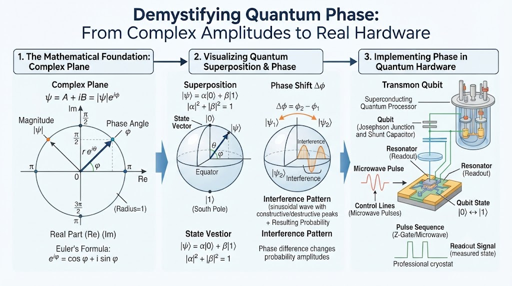
In quantum mechanics, a qubit does not behave merely as a point-like particle; its physical state is described mathematically by a wave function $\psi$. The quantum state of a single-qubit system is represented as a complex state vector in Hilbert space:
$$\vert{}\psi\rangle = \alpha \vert{}0\rangle + \beta \vert{}1\rangle$$
Here, $\vert{}0\rangle$ and $\vert{}1\rangle$ represent the standard computational basis states, while $\alpha$ and $\beta$ are complex numbers called probability amplitudes. Because $\alpha$ and $\beta$ are complex numbers, each can be expressed in polar form using Euler’s formula ($e^{i\phi} = \cos\phi + i\sin\phi$):
$$\alpha = r_0 e^{i\phi_0}, \quad \beta = r_1 e^{i\phi_1}$$
The parameters $\phi_0$ and $\phi_1$ represent the phase angles associated with the respective computational basis states. Quantum phase is the angular orientation of these complex probability amplitudes. It dictates how the underlying quantum wave functions interact when modified by quantum logic gates.
Why Quantum Phase Matters
If quantum computers only stored and manipulated magnitudes ($r_0$ and $r_1$), they would behave similarly to classical probabilistic algorithms, such as Markov chains or Monte Carlo simulations. In classical probability, probabilities are real numbers constrained between $0$ and $1$, and they always add up constructively:
$$P_{\text{total}} = P_1 + P_2$$
In quantum mechanics, probabilities are calculated by taking the squared magnitude of complex amplitudes:
$$P(x) = \vert{}\psi(x)\vert{}^2$$
Because quantum states are composed of complex numbers containing phase information, when two quantum computational paths overlap, their probability amplitudes add together before taking the squared magnitude:
$$\psi_{\text{total}} = \psi_1 + \psi_2$$
$$P_{\text{total}} = \vert{}\psi_1 + \psi_2\vert{}^2 = \vert{}\psi_1\vert{}^2 + \vert{}\psi_2\vert{}^2 + 2\vert{}\psi_1\vert{}\vert{}\psi_2\vert{}\cos(\Delta\phi)$$
     Classical Probabilities                 Quantum Amplitudes

         [ P1 ]   [ P2 ]                     [ ψ1 = r1 e^(iφ1) ]
           \       /                             \       /
            \     /                               \     /
         P_total = P1 + P2                 ψ_total = ψ1 + ψ2
    (Always increases/accumulates)            P_total = |ψ1 + ψ2|²
                                           (Can amplify OR cancel out!)
The term $2\vert{}\psi_1\vert{}\vert{}\psi_2\vert{}\cos(\Delta\phi)$ is the interference term, where $\Delta\phi = \phi_1 – \phi_0$ represents the difference in phase.
- If $\Delta\phi = 0$ (in phase), $\cos(0) = 1$, causing constructive interference that increases the likelihood of measuring a specific output.
- If $\Delta\phi = \pi$ ($180^\circ$ out of phase), $\cos(\pi) = -1$, causing destructive interference that suppresses the likelihood of that output down to zero.
Without quantum phase, quantum interference would not exist. Without interference, quantum computing would lack its primary computational mechanism, losing the ability to solve complex problems exponentially faster than classical systems.
Understanding Wave Functions and Probability Amplitudes
To build a solid operational framework, we must examine how quantum states are represented mathematically. The state vector $\vert{}\psi\rangle$ of a single qubit normalized to unity ($\vert{}\alpha\vert{}^2 + \vert{}\beta\vert{}^2 = 1$) can be written generally as:
$$\vert{}\psi\rangle = e^{i\gamma} \left( \cos\left(\frac{\theta}{2}\right) \vert{}0\rangle + e^{i\phi} \sin\left(\frac{\theta}{2}\right) \vert{}1\rangle \right)$$
This expression reveals three structural variables:
- $\theta$ (Theta): Controls the relative magnitude between $\vert{}0\rangle$ and $\vert{}1\rangle$, determining the raw measurement probabilities in the computational basis.
- $\gamma$ (Gamma): Represents the global phase factor of the quantum state.
- $\phi$ (Phi): Represents the relative phase shift between the $\vert{}0\rangle$ and $\vert{}1\rangle$ basis states.
                  Complex Plane Representation

                             +i (Imaginary)
                              |
                              |      * Amplitude β = r1 * e^(iφ)
                              |     /|
                              |    / |
                              |   /  |
                              |  /   |  r1 sin(φ)
                              | /    |
                              |/ φ   |
      ------------------------+------------------------ +r (Real)
                             /| r1 cos(φ)
                            / |
                           /  |
The probability of obtaining a specific output state upon measurement is governed by Born’s Rule:
$$P(\vert{}0\rangle) = \vert{}\alpha\vert{}^2 = \cos^2\left(\frac{\theta}{2}\right)$$
$$P(\vert{}1\rangle) = \vert{}\beta\vert{}^2 = \sin^2\left(\frac{\theta}{2}\right)$$
While direct measurement in the computational $Z$-basis ($\{\vert{}0\rangle, \vert{}1\rangle\}$) yields results that depend only on $\theta$, the relative phase angle $\phi$ dictates how the quantum state behaves when transformed by quantum gates prior to measurement.
Global Phase vs. Relative Phase
A common point of confusion when learning quantum mechanics is the difference between global phase and relative phase.
Global Phase
A global phase factor is a complex exponential $e^{i\gamma}$ that multiplies the entire state vector uniformally:
$$\vert{}\psi’\rangle = e^{i\gamma} \vert{}\psi\rangle = e^{i\gamma} (\alpha \vert{}0\rangle + \beta \vert{}1\rangle) = e^{i\gamma}\alpha \vert{}0\rangle + e^{i\gamma}\beta \vert{}1\rangle$$
Applying Born’s Rule to calculate the measurement probabilities of state $\vert{}\psi’\rangle$:
$$P(\vert{}0\rangle) = \vert{}e^{i\gamma}\alpha\vert{}^2 = (e^{i\gamma}\alpha)(e^{-i\gamma}\alpha^*) = e^0 \vert{}\alpha\vert{}^2 = \vert{}\alpha\vert{}^2$$
Because $e^{i\gamma}e^{-i\gamma} = 1$, the global phase factor cancels out completely during measurement. It produces no physically observable effects and cannot alter the outcome of any quantum experiment or algorithm. Therefore, quantum states that differ only by a global phase are physically indistinguishable:
$$\vert{}\psi\rangle \equiv e^{i\gamma} \vert{}\psi\rangle$$
Relative Phase
A relative phase angle $\phi$ is an internal phase difference between distinct basis components within a superposition state:
$$\vert{}\psi\rangle = \frac{1}{\sqrt{2}} \vert{}0\rangle + \frac{1}{\sqrt{2}} e^{i\phi} \vert{}1\rangle$$
Unlike global phase, relative phase cannot be factored out of the system. It fundamentally changes the physical properties of the quantum state, determining how it interacts with subsequent operations and interference pathways.
| Characteristic | Global Phase (eiγ) | Relative Phase (eiϕ) |
| Mathematical Form | $e^{i\gamma}(\alpha\vert{}0\rangle + \beta\vert{}1\rangle)$ | $\alpha\vert{}0\rangle + e^{i\phi}\beta\vert{}1\rangle$ |
| Physical Significance | Unobservable; no physical impact | Observable; drives quantum interference |
| Measurement Impact ($Z$-basis) | Identical probability outcomes | Identical outcomes in $Z$, different in $X/Y$ |
| Bloch Sphere Effect | No physical movement | Rotates vector around the $Z$-axis |
| Algorithmic Utility | None | Core driver of quantum speedups |
How Quantum Phase Affects Qubits
To see how relative phase changes a qubit’s physical state, consider two normalized superposition states:
$$\vert{}+\rangle = \frac{1}{\sqrt{2}}\vert{}0\rangle + \frac{1}{\sqrt{2}}\vert{}1\rangle \quad (\phi = 0)$$
$$\vert{}-\rangle = \frac{1}{\sqrt{2}}\vert{}0\rangle – \frac{1}{\sqrt{2}}\vert{}1\rangle \quad (\phi = \pi, \text{ since } e^{i\pi} = -1)$$
If we measure both states in the standard computational basis ($Z$-basis), both return $\vert{}0\rangle$ with 50% probability and $\vert{}1\rangle$ with 50% probability:
$$P_{\vert{}+\rangle}(0) = \left\vert{}\frac{1}{\sqrt{2}}\right\vert{}^2 = 0.5, \quad P_{\vert{}+\rangle}(1) = \left\vert{}\frac{1}{\sqrt{2}}\right\vert{}^2 = 0.5$$
$$P_{\vert{}-\rangle}(0) = \left\vert{}\frac{1}{\sqrt{2}}\right\vert{}^2 = 0.5, \quad P_{\vert{}-\rangle}(1) = \left\vert{}-\frac{1}{\sqrt{2}}\right\vert{}^2 = 0.5$$
Based solely on computational basis measurements, $\vert{}+\rangle$ and $\vert{}-\rangle$ appear identical. However, applying a Hadamard gate ($H$) to both states prior to measurement reveals their operational differences:
$$H = \frac{1}{\sqrt{2}} \begin{pmatrix} 1 & 1 \\ 1 & -1 \end{pmatrix}$$
Applying $H$ to $\vert{}+\rangle$:
$$H\vert{}+\rangle = \frac{1}{\sqrt{2}} \begin{pmatrix} 1 & 1 \\ 1 & -1 \end{pmatrix} \begin{pmatrix} \frac{1}{\sqrt{2}} \\ \frac{1}{\sqrt{2}} \end{pmatrix} = \begin{pmatrix} 1 \\ 0 \end{pmatrix} = \vert{}0\rangle$$
Applying $H$ to $\vert{}-\rangle$:
$$H\vert{}-\rangle = \frac{1}{\sqrt{2}} \begin{pmatrix} 1 & 1 \\ 1 & -1 \end{pmatrix} \begin{pmatrix} \frac{1}{\sqrt{2}} \\ -\frac{1}{\sqrt{2}} \end{pmatrix} = \begin{pmatrix} 0 \\ 1 \end{pmatrix} = \vert{}1\rangle$$
   Relative Phase Determines Outcome After Basis Change:

   |+⟩ State (φ = 0)   ───► [ H Gate ] ───► Deterministically yields |0⟩

   |-⟩ State (φ = π)   ───► [ H Gate ] ───► Deterministically yields |1⟩
The relative phase difference ($\Delta\phi = \pi$) converts what appeared to be identical classical probabilities into completely deterministic opposite outcomes ($\vert{}0\rangle$ vs. $\vert{}1\rangle$). This demonstrates that phase stores real, accessible quantum information.
Phase and Quantum Superposition
Quantum superposition is often described simply as “being in multiple states at once.” However, a more precise definition is that superposition is a coherent linear combination of basis states with well-defined phase relationships.
Superposition without Phase Control = Incoherent Mixture (Noise)
Superposition with Precise Phase Control = Functional Quantum State
If the phase relationship between $\vert{}0\rangle$ and $\vert{}1\rangle$ fluctuates randomly due to environmental noise, the state undergoes dephasing (loss of phase coherence). A dephased quantum state transitions from a coherent superposition into an incoherent probabilistic mixture described by a reduced density matrix:
$$\rho = \begin{pmatrix} \vert{}\alpha\vert{}^2 & 0 \\ 0 & \vert{}\beta\vert{}^2 \end{pmatrix}$$
When phase coherence is lost, the qubit loses its ability to perform interference, behaving instead like a classical probabilistic bit. Maintaining precise phase relationships within a superposition is therefore essential for running quantum algorithms.
Quantum Interference Explained
Quantum interference is the operational engine of quantum algorithms. It allows a quantum computer to evaluate millions of possibilities simultaneously while using phase relationships to direct the system toward the correct solution.
                          QUANTUM INTERFERENCE MECHANISM

      Initial Superposition         Phase Shift Applied         Hadamard Transform
     ┌─────────────────────┐       ┌───────────────────┐       ┌───────────────────┐
     │  Path A: +0.50 |00⟩ │  ───► │  Path A: +0.50|00⟩│  ───► │ Constructive:     │
     │  Path B: +0.50 |01⟩ │       │  Path B: +0.50|01⟩│       │ 100% Signal on    │
     │  Path C: +0.50 |10⟩ │       │  Path C: -0.50|10⟩│       │ Correct Answer    │
     │  Path D: +0.50 |11⟩ │       │  Path D: +0.50|11⟩│       │                   │
     └─────────────────────┘       └───────────────────┘       │ Destructive:      │
                                    (Sign Flip on C)           │ 0% Signal on      │
                                                               │ Wrong Answers     │
                                                               └───────────────────┘
Consider how Grover’s Search Algorithm uses phase to find an item in an unsorted database:
- Initialization: Prepare an equal superposition of all possible $N$ items using Hadamard gates. Every state shares the exact same amplitude and relative phase.
- Oracle Application (Phase Inversion): The quantum oracle identifies the target state $\vert{}x_{target}\rangle$ and flips its phase by $180^\circ$ ($e^{i\pi} = -1$), leaving all non-target states unchanged.
- Amplification (Reflection about the Mean): A diffusion operator uses this phase difference to perform constructive interference on the target state while causing destructive interference on the incorrect states.
- Measurement: Measuring the system returns the target state with near-certainty.
By manipulating phases rather than searching sequentially, Grover’s algorithm achieves a quadratic speedup $O(\sqrt{N})$ over classical search methods $O(N)$.
Phase Shift Gates
Quantum hardware performs phase operations using single-qubit unitary phase shift gates. These gates leave the $\vert{}0\rangle$ state unchanged while rotating the phase angle of the $\vert{}1\rangle$ component.
   Generic Phase Gate Operation:

   |0⟩ ───────────────────► |0⟩
   |1⟩ ───[ Phase Shift ]─► e^(iθ) |1⟩
The general matrix representation of a Phase Shift Gate $R_\lambda$ is:
$$P(\lambda) = R_\lambda = \begin{pmatrix} 1 & 0 \\ 0 & e^{i\lambda} \end{pmatrix}$$
Core Single-Qubit Phase Gates
1. Pauli-Z Gate ($\pi$ Phase Shift)
Flips the sign of the $\vert{}1\rangle$ state ($180^\circ$ rotation around the $Z$-axis of the Bloch sphere):
$$Z = \begin{pmatrix} 1 & 0 \\ 0 & -1 \end{pmatrix}$$
$$Z\vert{}0\rangle = \vert{}0\rangle, \quad Z\vert{}1\rangle = -\vert{}1\rangle$$
2. S Gate ($\pi/2$ Phase Shift / Phase Gate)
Applies a $90^\circ$ phase shift to the $\vert{}1\rangle$ state. It is the square root of the $Z$ gate ($S^2 = Z$):
$$S = \begin{pmatrix} 1 & 0 \\ 0 & i \end{pmatrix} = \begin{pmatrix} 1 & 0 \\ 0 & e^{i\pi/2} \end{pmatrix}$$
3. T Gate ($\pi/4$ Phase Shift / $\pi/8$ Gate)
Applies a $45^\circ$ phase shift to the $\vert{}1\rangle$ state. It is the square root of the $S$ gate ($T^2 = S$). The $T$ gate is non-Clifford, making it critical for achieving universal fault-tolerant quantum computing:
$$T = \begin{pmatrix} 1 & 0 \\ 0 & e^{i\pi/4} \end{pmatrix} = \begin{pmatrix} 1 & 0 \\ 0 & \frac{1+i}{\sqrt{2}} \end{pmatrix}$$
4. Arbitrary Rotation Gate $RZ(\theta)$
Rotates the quantum state by an arbitrary angle $\theta$ around the $Z$-axis:
$$RZ(\theta) = \exp\left(-i \frac{\theta}{2} Z\right) = \begin{pmatrix} e^{-i\theta/2} & 0 \\ 0 & e^{i\theta/2} \end{pmatrix}$$
Phase in Quantum Circuits
In multi-qubit circuits, quantum phase can be dynamically passed between qubits using controlled gate operations. This mechanism is known as Phase Kickback.
                           PHASE KICKBACK CIRCUIT

  Control: |+⟩  ────■───────────── |0⟩ + e^(iφ)|1⟩  (Phase kicked back!)
                    │              ───────────────
                    │                    √2
  Target:  |u⟩  ──[ U ]─────────── e^(iφ)|u⟩        (Eigenstate preserved)
Phase kickback occurs when a controlled-unitary operation $C-U$ is applied to a target qubit set to an eigenstate $\vert{}u\rangle$ of $U$, where $U\vert{}u\rangle = e^{i\phi}\vert{}u\rangle$:
- The control qubit is prepared in a superposition $\vert{}+\rangle = \frac{1}{\sqrt{2}}(\vert{}0\rangle + \vert{}1\rangle)$.
- The combined system state is:$$\vert{}\psi_0\rangle = \frac{1}{\sqrt{2}}(\vert{}0\rangle + \vert{}1\rangle) \otimes \vert{}u\rangle = \frac{1}{\sqrt{2}}(\vert{}0\rangle\vert{}u\rangle + \vert{}1\rangle\vert{}u\rangle)$$
- Applying the $C-U$ operation transforms the state:$$\vert{}\psi_1\rangle = \frac{1}{\sqrt{2}}(\vert{}0\rangle\vert{}u\rangle + \vert{}1\rangle U\vert{}u\rangle) = \frac{1}{\sqrt{2}}(\vert{}0\rangle\vert{}u\rangle + e^{i\phi}\vert{}1\rangle\vert{}u\rangle)$$
- Factoring out the target eigenstate $\vert{}u\rangle$ gives:$$\vert{}\psi_1\rangle = \left( \frac{\vert{}0\rangle + e^{i\phi}\vert{}1\rangle}{\sqrt{2}} \right) \otimes \vert{}u\rangle$$
The eigenvalue phase factor $e^{i\phi}$ generated by the target qubit has been kicked back onto the control qubit as a relative phase shift. Phase kickback is the primary building block for advanced algorithms like Quantum Phase Estimation.
Quantum Phase Estimation (QPE)
Quantum Phase Estimation (QPE) is a foundational subroutine in quantum computing. It solves a direct problem: given a unitary operator $U$ and an eigenstate $\vert{}u\rangle$ such that $U\vert{}u\rangle = e^{2\pi i \theta}\vert{}u\rangle$, QPE estimates the phase parameter $\theta$ (where $0 \le \theta < 1$).
                 QUANTUM PHASE ESTIMATION CIRCUIT SCHEMATIC

  Counting Register (n qubits)
  |0⟩ ───[ H ]──────■─────────────────────────┐
  |0⟩ ───[ H ]──────┼─────────■───────────────┼───[   QFT†   ]─── Measure ──► Phase θ
  |0⟩ ───[ H ]──────┼─────────┼─────────■─────┤   Inverse    │    Binary: .θ1θ2...θn
                    │         │         │     │  Transform   │
  Target Register   │2^(n-1)  │2^1      │2^0  └──────────────┘
  |u⟩ ────────────[ U ]─────[ U ]─────[ U ]───────────────────── Keep |u⟩
Operational Steps of QPE:
- Register Setup: Initialize an $n$-qubit counting register in the state $\vert{}0\rangle^{\otimes n}$ alongside a target register containing eigenstate $\vert{}u\rangle$.
- Superposition: Apply Hadamard gates to all $n$ counting qubits to create an equal superposition.
- Controlled Operations & Phase Kickback: Apply a series of controlled-$U^{2^j}$ operations from the counting qubits to the target register. Through phase kickback, phase shifts are written directly into the counting register:$$\frac{1}{2^{n/2}} \sum_{k=0}^{2^n-1} e^{2\pi i \theta k} \vert{}k\rangle \otimes \vert{}u\rangle$$
- Inverse Quantum Fourier Transform ($QFT^\dagger$): Apply $QFT^\dagger$ to convert the phase stored in the complex amplitudes of the counting register into a binary computational state $\vert{}\theta_1 \theta_2 \dots \theta_n\rangle$.
- Measurement: Read out the counting register to obtain an $n$-bit binary approximation of the phase $\theta$.
QPE provides the core acceleration behind quantum algorithms for chemistry, materials science, and cryptography.
Phase in Quantum Algorithms
Quantum phase is central to many major quantum algorithms.
                   QUANTUM ALGORITHMS PHASE DEPENDENCY

    ┌──────────────────────────┐         ┌──────────────────────────┐
    │ Quantum Fourier          │         │ Shor's Factoring         │
    │ Transform (QFT)          │ ──────► │ Algorithm                │
    │ Maps Basis -> Phase      │         │ Finds Order via Phase    │
    └──────────────────────────┘         └──────────────────────────┘
                 │                                    │
                 ▼                                    ▼
    ┌──────────────────────────┐         ┌──────────────────────────┐
    │ Quantum Phase            │         │ HHL Linear Systems       │
    │ Estimation (QPE)         │ ──────► │ Algorithm                │
    │ Measures Eigenphases     │         │ Extracts Eigenvalues     │
    └──────────────────────────┘         └──────────────────────────┘
1. The Quantum Fourier Transform (QFT)
The QFT is the quantum equivalent of the classical Discrete Fourier Transform. It maps a quantum state from the computational basis into the phase/Fourier basis:
$$\text{QFT}\vert{}x\rangle = \frac{1}{\sqrt{N}} \sum_{y=0}^{N-1} e^{2\pi i x y / N} \vert{}y\rangle$$
While the classical Fast Fourier Transform (FFT) requires $O(N 2^N)$ operations, the QFT runs in $O(n^2)$ gate operations for $n = \log_2 N$ qubits, providing an exponential speedup.
2. Shor’s Factoring Algorithm
Shor’s algorithm breaks RSA encryption by finding the period $r$ of the modular function $f(x) = a^x \pmod N$. Period finding is reduced to a phase estimation problem:
- The modular exponentiation function is encoded into a unitary operator $U_a \vert{}y\rangle = \vert{}ay \pmod N\rangle$.
- The eigenvalues of $U_a$ contain phase values proportional to $s/r$ (where $s$ is an integer).
- Applying QPE extracts the phase, enabling a classical computer to compute the period $r$ using continued fractions and factor the composite number $N$ in polynomial time.
Phase and Quantum Error Correction
In real-world quantum hardware, noise causes two primary types of physical errors:
- Bit-Flip Errors ($X$ Error): The qubit flips between state $\vert{}0\rangle$ and $\vert{}1\rangle$ (analogous to classical bit flips).
- Phase-Flip Errors ($Z$ Error): The relative phase flips sign ($\vert{}0\rangle + \vert{}1\rangle \rightarrow \vert{}0\rangle – \vert{}1\rangle$), corrupting the stored phase without altering the computational population.
                            TYPES OF QUANTUM NOISE

     Bit-Flip Noise (X)                      Phase-Flip Noise (Z)
   [ |0⟩ ] ──────► [ |1⟩ ]                |0⟩ + |1⟩ ──────► |0⟩ - |1⟩
   (Changes state population)             (Destroys relative phase angle)
Phase errors are particularly challenging because they cannot be detected by simply measuring computational probabilities in the $Z$-basis.
Protecting Against Phase Errors
To correct phase-flip errors, Quantum Error Correction (QEC) protocols (such as the Shor 9-qubit code or Surface Codes) map phase-flip errors into bit-flip errors using Hadamard transformations:
  Phase Error Circuit Protection:

  |ψ⟩ ──[ H ]──► [ Phase Noise Z ] ──[ H ]──► Bit-Flip Error X (Detectable!)
By changing basis ($H Z H = X$), the system converts phase errors into bit-flip errors, allowing ancilla qubits and syndrome measurements to detect and correct the noise without collapsing the underlying quantum information.
Visualizing Quantum Phase with the Bloch Sphere
The Bloch Sphere provides a geometric representation of a single qubit’s state space.
                                    |0⟩ (Z+)
                                     |
                                     |    |θ
                                     |   /
                                     |  /
                                     | /  Vector |ψ⟩
                                     |/__________ Y+
                                    / \
                                   /   \
                                  /     \  Phase Angle φ
                                 /       \
                              X+
                                     |
                                     |
                                    |1⟩ (Z-)
On the Bloch Sphere, any pure state vector is defined by two angles, $\theta$ and $\phi$:
$$\vert{}\psi\rangle = \cos\left(\frac{\theta}{2}\right)\vert{}0\rangle + e^{i\phi}\sin\left(\frac{\theta}{2}\right)\vert{}1\rangle$$
- Polar Angle ($\theta$): Determines latitude (distance between $\vert{}0\rangle$ at the North Pole and $\vert{}1\rangle$ at the South Pole). It sets the measurement probabilities in the $Z$-basis.
- Azimuthal Angle ($\phi$): Determines longitude (rotation around the Equator in the $X$-$Y$ plane). This represents the relative phase angle.
How Gates Shift the Vector:
- $X$ Gate: Rotates the vector $180^\circ$ around the $X$-axis.
- $Z$ Gate: Rotates the vector $180^\circ$ around the $Z$-axis, changing $\phi \rightarrow \phi + \pi$.
- $S$ Gate: Rotates the vector $90^\circ$ around the $Z$-axis, changing $\phi \rightarrow \phi + \pi/2$.
- $T$ Gate: Rotates the vector $45^\circ$ around the $Z$-axis, changing $\phi \rightarrow \phi + \pi/4$.
Practical Examples Using Qiskit and IBM Quantum
Below is a complete, runnable code example using Qiskit 1.0+ that demonstrates how relative phase affects measurement outcomes.
Step 1: Install Qiskit
Bash
pip install qiskit qiskit-aer matplotlib
Step 2: Phase Manipulation Example
Python
import numpy as np
from qiskit import QuantumCircuit
from qiskit_aer import AerSimulator
from qiskit.visualization import plot_histogram

# Initialize simulator
simulator = AerSimulator()

# -------------------------------------------------------------
# Circuit A: Hadamard -> S Gate (pi/2 Phase Shift) -> Hadamard
# -------------------------------------------------------------
qc_a = QuantumCircuit(1, 1)
qc_a.h(0)         # Create |+> superposition state
qc_a.s(0)         # Apply S gate (injects pi/2 relative phase shift)
qc_a.h(0)         # Rotate back using Hadamard gate
qc_a.measure(0, 0)

# -------------------------------------------------------------
# Circuit B: Hadamard -> Z Gate (pi Phase Shift) -> Hadamard
# -------------------------------------------------------------
qc_b = QuantumCircuit(1, 1)
qc_b.h(0)         # Create |+> superposition state
qc_b.z(0)         # Apply Z gate (injects pi relative phase shift)
qc_b.h(0)         # Rotate back using Hadamard gate
qc_b.measure(0, 0)

# Execute Circuits
result_a = simulator.run(qc_a, shots=1000).result()
counts_a = result_a.get_counts()

result_b = simulator.run(qc_b, shots=1000).result()
counts_b = result_b.get_counts()

print("Results for Circuit A (S-gate phase shift):", counts_a)
print("Results for Circuit B (Z-gate phase shift):", counts_b)
Expected Output & Analysis:
- Circuit A Output: Returns approximately 50%
0and 50%1. The $S$ gate shifted the state vector to $\vert{}e_y+\rangle = \frac{1}{\sqrt{2}}(\vert{}0\rangle + i\vert{}1\rangle)$ along the $Y$-axis, producing an equal superposition after the second Hadamard transform. - Circuit B Output: Returns 100%
1({'1': 1000}). The $Z$ gate flipped the relative phase from $\vert{}+\rangle$ to $\vert{}-\rangle$. The final Hadamard transform then deterministically mapped $\vert{}-\rangle$ back to computational state $\vert{}1\rangle$.
Common Misconceptions About Quantum Phase
1. “Global Phase Can Be Measured Directly”
Fact: Global phase factors ($e^{i\gamma}$) drop out completely when calculating expectation values or measurement probabilities. They are physically unobservable. Only relative phase differences produce measurable physical effects.
2. “Phase Changes Modify Measurement Probabilities Immediately”
Fact: Applying a phase gate (like $Z, S, T$) to a state in the computational basis changes only its longitude on the Bloch sphere ($\phi$). The measurement probabilities in the $Z$-basis stay exactly $50/50$. To observe phase shifts as changed outcomes, you must first apply a basis-changing gate (such as $H$).
3. “Quantum Phase and Classical Phase are Identical”
Fact: While both use similar wave mathematics, classical phase describes physical wave offsets in spatial media or fields. Quantum phase exists within abstract complex probability amplitudes in multi-dimensional Hilbert spaces, enabling non-classical phenomena like entanglement and phase kickback.
Real-World Applications of Phase-Based Quantum Computing
                  REAL-WORLD APPLICATIONS OF QUANTUM PHASE

    ┌──────────────────────────┐         ┌──────────────────────────┐
    │ Quantum Chemistry        │         │ Cryptography & Security  │
    │ Simulates Molecular      │         │ Breaks RSA via Shor's;   │
    │ Binding & Energy Levels  │         │ Enables Post-Quantum Crypto│
    └──────────────────────────┘         └──────────────────────────┘
                 │                                    │
                 ▼                                    ▼
    ┌──────────────────────────┐         ┌──────────────────────────┐
    │ Quantum Sensing          │         │ Financial Modeling       │
    │ Measures Magnetic/Gravity│         │ Accelerates Monte Carlo  │
    │ Fields via Interferometry│         │ Risk Calculations (QAE) │
    └──────────────────────────┘         └──────────────────────────┘
- Quantum Chemistry and Materials Simulation: Variational Quantum Eigensolvers (VQE) and Phase Estimation algorithms calculate electronic ground states and molecular binding energies by resolving subtle quantum phases in complex wave functions.
- Quantum Sensing and Metrology: Quantum sensors use phase interferometry to measure magnetic fields, gravitational gradients, and time standards with sensitivity far beyond classical limits.
- Financial Risk Analysis: Quantum Amplitude Estimation (QAE)—which builds directly on Quantum Phase Estimation—speeds up classical Monte Carlo simulations for financial risk analysis, option pricing, and portfolio optimization.
- Post-Quantum Cryptography & Security: Understanding how phase estimation cracks classical asymmetric encryption (RSA, ECC) helps security architects transition systems to lattice-based post-quantum cryptography.
Current Challenges in Phase Control
Controlling quantum phase in real hardware requires precise physical manipulation. Modern quantum systems face several challenges:
- Dephasing ($T_2$ Coherence Time): Environmental interactions (such as thermal noise, electromagnetic fluctuations, or stray magnetic fields) degrade relative phase over time, limiting circuit depth.
- Control Crosstalk: Applying a phase gate to one qubit can inadvertently cause unwanted phase shifts in neighboring qubits.
- Phase Drift: Microwave control pulses and laser sources used in trapped-ion and superconducting platforms drift over time, requiring continuous calibration.
Future of Phase Engineering in Quantum Systems
As the industry transitions from Noise Intermediate-Scale Quantum (NISQ) devices to Fault-Tolerant Quantum Computing (FTQC), phase control remains a key focus:
- Composite & Refocused Pulse Sequences: Advanced pulse design (such as dynamical decoupling) actively shields qubits from phase noise.
- Fault-Tolerant T-Factory Distillation: Because $T$ gates inject non-Clifford phase shifts ($\pi/4$), generating pure $T$-states through state distillation is central to fault-tolerant hardware architectures.
- Analogue Quantum Simulators: Programmable neutral-atom arrays leverage phase control to simulate complex quantum materials directly.
Learning Roadmap for Beginners
To master quantum phase, quantum algorithms, and QuantumOps, follow this structured learning path:
                  QUANTUM PHASE LEARNING ROADMAP

  Stage 1: Math Foundations  ──► Linear Algebra, Complex Numbers, Dirac Notation
  Stage 2: Single Qubit Gate ──► Bloch Sphere, Z/S/T Gates, Superposition
  Stage 3: Multi-Qubit Systems──► Entanglement, Phase Kickback, Controlled Gates
  Stage 4: Core Algorithms   ──► QFT, Quantum Phase Estimation, Grover Search
  Stage 5: Hands-On Code     ──► Qiskit, OpenQASM 3, IBM Quantum Cloud Execution
  Stage 6: QuantumOps        ──► Circuit Optimization, Noise Mitigation, Deployments
- Step 1: Mathematical PrerequisitesMaster linear algebra, complex vectors, matrix operations, Euler’s formula, and Dirac bra-ket notation.
- Step 2: Single-Qubit MechanicsStudy the Bloch sphere, basis changes, and basic single-qubit gates ($H, X, Z, S, T$).
- Step 3: Multi-Qubit Circuits & KickbackLearn controlled operations ($CNOT, CZ, CU$), entanglement, and the phase kickback mechanism.
- Step 4: Algorithm Deep DivesWork through the Quantum Fourier Transform, Quantum Phase Estimation, Grover’s search, and Shor’s algorithm.
- Step 5: Practical CodingBuild, simulate, and execute quantum circuits on real quantum hardware using Qiskit and OpenQASM 3.
- Step 6: QuantumOps Best PracticesLearn circuit transpilation, error mitigation strategies, noise profiling, and production deployment pipelines.
Career Opportunities in Quantum Computing
As quantum technologies mature, demand is growing across several roles:
- Quantum Software Engineer: Designs, optimizes, and implements quantum circuits and algorithms.
- Quantum Algorithm Researcher: Develops new algorithms for quantum chemistry, machine learning, and optimization problems.
- QuantumOps / Platform Engineer: Manages hybrid classical-quantum cloud integrations, circuit compilation pipelines, and job execution workflows.
- Quantum Hardware / Control Engineer: Works on pulse-level control, microwave engineering, and phase-calibration software for quantum processors.
Frequently Asked Questions (FAQs)
What is quantum phase in simple terms?
Quantum phase is the angular position or cycle state of a quantum system’s wave function. It acts as an internal clock that dictates how quantum states interfere with one another.
Can we measure quantum phase directly?
No. Direct measurement in the computational basis ($Z$-basis) collapses the quantum state and reveals only magnitude probabilities. To measure phase, you must first apply basis-changing operations (like a Hadamard gate) to convert relative phase shifts into measurable probability differences.
What is the difference between global phase and relative phase?
Global phase shifts the entire quantum state uniformly ($e^{i\gamma}\vert{}\psi\rangle$) and produces no physically observable effects. Relative phase is a phase difference between distinct superposition basis states ($\alpha\vert{}0\rangle + e^{i\phi}\beta\vert{}1\rangle$), directly driving quantum interference and algorithmic operations.
Why are S and T gates important for quantum phase?
The $S$ gate ($\pi/2$ phase shift) and $T$ gate ($\pi/4$ phase shift) provide fine-grained control over a qubit’s phase angle. The $T$ gate is non-Clifford, making it essential for fault-tolerant, universal quantum computing.
What is phase kickback?
Phase kickback is a quantum circuit mechanism where applying a controlled-unitary gate to a target qubit in an eigenstate writes the resulting phase eigenvalue directly back onto the control qubit as a relative phase shift.
How does phase enable quantum interference?
Relative phase determines whether overlapping quantum probability amplitudes add together constructively (increasing the probability of that outcome) or subtract destructively (canceling the outcome out).
What is Quantum Phase Estimation (QPE)?
QPE is a core quantum algorithm used to estimate the unknown phase angle $\theta$ associated with an eigenvalue of a unitary operator $U|u\rangle = e^{2\pi i \theta}|u\rangle$. It is a central building block for Shor’s algorithm and quantum chemistry simulations.
What is dephasing in quantum computing?
Dephasing is a form of quantum noise where environmental interactions cause a qubit to lose its relative phase coherence over time ($T_2$ relaxation). This destroys superposition and converts the qubit into an incoherent classical state.
How does Qiskit manipulate quantum phase?
Qiskit provides built-in gate operations—such as qc.z(), qc.s(), qc.t(), qc.rz(theta), and qc.p(lambda)—that alter a qubit’s relative phase angle directly within a quantum circuit.
What is the role of phase in Shor’s algorithm?
Shor’s algorithm uses Quantum Phase Estimation to find the period of a modular function. The period is extracted from the eigenphase of a modular multiplication operator, enabling the algorithm to factor large integers efficiently.
Conclusion
Quantum phase is a cornerstone of quantum computing. Far from being a mere mathematical detail, relative phase enables quantum superposition, drives quantum interference, powers key algorithms like QPE and Shor’s algorithm, and underpins quantum error correction. As quantum hardware scales and QuantumOps practices mature, precise control over quantum phase remains critical to achieving functional quantum advantage. Understanding how to manipulate phase within quantum circuits is an essential step for developers, engineers, and researchers entering the field of quantum technology.